从 Partial CUDA Graph 到 Full CUDA Graph
在上一篇深入理解 Megatron-LM 中的 Partial CUDA Graph:MoE 模型训练加速的关键技术中,我们分析了 MoE 训练流程中影响 CUDA Graph 兼容性的主要瓶颈在于 MoE 部分的动态行为 —— 每个 expert 在每次 iteration 中接收的 token 数量都不同,导致 kernel 参数、缓冲区大小和通信模式无法在捕获时固定。 本文将深入探讨如何逐一攻克这些障碍,使 MoE 部分能够无缝融入 CUDA Graph,并最终实现覆盖前向与反向传播的完整 iteration 的 Full CUDA Graph 捕获。与 Partial CUDA Graph(仅捕获 Attention、MLP 等确定性模块)不同,Full CUDA Graph 会将整个训练 iteration(包括 MoE 层)作为一个完整的 GPU 执行图进行捕获和重放,从而最大程度地消除 CPU 开销。 为了解决 MoE 与 CUDA Graph 的兼容性,首先需要攻克以下两个核心技术难题:
- 消除 TE grouped GEMM 中的 CPU-GPU 同步:当前 TE 在启动 grouped GEMM 时依赖
torch.split,该操作要求将 GPU 上的tokens_per_expert转移至 CPU,这会触发隐式同步,破坏 CUDA Graph 的捕获流程。 - 重构 HybridEP 策略以兼容 CUDA Graph:HybridEP 的 token 分发逻辑仍包含动态内存分配和条件分支,需要重构为静态缓冲区 + 固定执行路径模式。这一点其实在 HybridEP 2025 年底的几个 commit 中都有所涉及,我们可以认为现在的 HybridEP 版本已经兼容 CUDA Graph 了。
实际上,完成上述两项优化后,在 MoE 强制负载均衡(force load balancing)设定下,已经可以实现真正意义上的 Full CUDA Graph。然而,在实际训练中并不会采用 force load balancing;而由于 CUDA Graph 需要静态特性,我们也无法在每个 EP Rank 上为极端不均衡的情况预留过大的缓冲区。因此,我们还需要结合 MoE 的负载均衡算法,并实现高效的 Expert 权重分发与梯度聚合机制,同时保持与 CUDA Graph 的兼容,以便在真实场景下安全、高效地使用 Full CUDA Graph。
在接下来的内容中,我们会调整行文顺序:先讨论 CUDA Graph 兼容的 MoE 负载均衡算法,再讨论如何实现高效的 Expert 权重分发与梯度聚合机制,接着介绍 Megatron Full CUDA Graph 的整体实现机制,最后介绍如何解决 TE grouped GEMM 的 CPU-GPU 同步问题。
MoE 负载规划算法
为了实现 MoE 的负载均衡,我们引入了 redundant expert slots(冗余专家槽位)的概念。每个 EP rank 需要预先分配固定数量的 expert 计算槽位。当某些 EP rank 的负载过重(即分配到的 token 数远超平均值)时,可以将部分 token offload 到负载较轻的 EP rank 的空闲槽位上处理。这就需要一套机制来决定:哪些 expert 的权重需要被复制到哪些 redundant expert slots 上,这个机制我们称之为 expert dispatch。我们可以在后文中看到,实际上 expert dispatch 和 token dispatch 非常像,甚至都可以复用 HybridEP 这套通信库。
下图展示了前向过程中整个 expert dispatch 和 token dispatch 的工作流程:
sequenceDiagram
    participant Input as Hidden States
    participant Router
    participant Planner as Offloading Planner
    participant ExpertDisp as Expert Dispatcher
    participant TokenDisp as Token Dispatcher
    participant Experts
    participant Output

    Input->>Router: hidden_states
    Router->>Planner: routing_map, probs
    Planner->>Planner: gen_offloading_plan()
    Planner->>ExpertDisp: expert_offloading_map
    ExpertDisp->>Experts: dispatch weights to echo experts
    Input->>TokenDisp: hidden_states, rerouted_probs
    TokenDisp->>Experts: dispatched tokens
    Experts->>TokenDisp: expert outputs
    TokenDisp->>Output: combined output
假设现在我们已经有了一个 router 生成的路由方案,即我们知道每个 EP rank 上每个 home expert 会收到多少 token。我们现在要做 MoE 的负载规划,即决定每个 EP rank 上的每个 home expert 要将其权重分发到哪个 EP rank 的 redundant expert slots 上,并同时决定原本路由到该 home expert 的 token 中有多少要改为路由到这个 redundant expert slot 上。 这里有三个层级的考虑:
- 第一个层级是要考虑每个 EP Rank 上的空闲容量(spare capacity)。空闲容量表示一个 EP rank 还能额外处理多少 token,我们肯定不能将太多的 token 重路由到一个 EP rank 上,我们希望转移后每个 EP Rank 上的计算量更加均衡。
- 第二个层级是 home expert 上的,我们想要计算每个 home expert 的溢出量(spillover)。溢出量表示一个 home expert 有多少 token 需要被转移到其他 EP rank 上处理,在这个层级我们希望尽可能减少 expert 权重分发的通信量。比如说,假设某个 home expert 只被安排了转移 1 个 token 的计算到其他 redundant expert slot 上,但是我们却需要将整个 expert 权重分发到这个 redundant expert slot 上,显然这是非常不合算的。
- 第三个层级是专家权重的分配。有了每个 EP rank 的 spare capacity 和每个 home expert 的 spillover 之后,每个 home expert 的权重应该被分配到哪个 EP rank 的 spare slot 上。
我们一步步来解决这些问题。
基于前缀和的分摊算法
我们在这一节中考虑第一层级和第二层级的事情。首先考虑每个 EP rank 上的 spare capacity 如何计算:
def gen_intermediate(count_tokens_per_expert_from_ep_rank, ...):
    # 步骤1: 计算每个EP rank的token总数和平均值
    count_tokens_per_ep_rank = count_tokens_per_expert.view(num_ep_ranks, -1).sum(dim=1)
    avg_tokens_per_ep_rank = count_tokens_per_ep_rank.sum() // num_ep_ranks

    # 步骤2: 计算spare容量 = max(0, avg - current)
    # 负载低于平均的EP rank有空闲容量接收tokens
    deviation = count_tokens_per_ep_rank - avg_tokens_per_ep_rank
    capacity_spare_per_ep_rank = torch.relu(-deviation)

    # 步骤3: 计算spillover(溢出量)
    # 关键思路:对每个EP rank内的专家按token数排序,
    # 累积求和后超过平均值的部分就是spillover
    count_tokens_sorted, indices_sorted = count_tokens_per_expert.view(num_ep_ranks, -1).sort(dim=1)
    spillover_cumsum = (count_tokens_sorted.cumsum(dim=1) - avg_tokens_per_ep_rank).clamp(min=0)
    # 从cumsum转回每个专家的spillover
    count_spillover_sorted = torch.cat([spillover_cumsum[:, :1],
                                         torch.diff(spillover_cumsum, dim=1)], dim=1)
空闲容量的计算非常简单:超过均值的部分要转移到其他 EP rank,没有达到均值的 EP rank 就有空闲容量来承载转移。下面通过一个直观的例子来理解:假设有 4 个 EP ranks,每个 EP rank 上有 4 个 home experts(共 16 个 experts,编号 0-15),token 总数为 1000,平均每个 EP rank 应处理 250 个 token:
                avg = 250
                    │
EP0: 500 ■■■■■■■■■■│■■■■■■■■■■  超额 250 → 转移到其他EP rank
EP1: 350 ■■■■■■■   │■■■           超额 100 → 转移到其他EP rank
EP2: 100 ■■        │              空闲 150 → spare capacity
EP3:  50 ■         │              空闲 200 → spare capacity
                    │
现在我们知道了每个 EP rank 整体需要 offload 多少 token。接下来考虑第二个问题:如何设计一种分摊算法,将 EP rank 层级的溢出量分摊到各个 expert 上,使得各 expert 的 spillover 之和恰好等于该 EP rank 的总溢出量? 注意在这个问题里面,我们希望将 expert 权重分发的代价尽可能小,尽可能不要出现分发了一次 expert 权重但是只为了转移一个 token 的情况。
为此,我们算法设计的思想是:负载较轻的专家优先保留自己的 tokens,而负载较重的专家承担更多的 spillover。分摊算法如下:以上面的 EP0 为例,假设其有 4 个 experts(编号 0-3),tokens 分布为 [50, 100, 150, 200](总和 500),avg_tokens_per_ep_rank 为 250:
# Step 1: 排序(从小到大)
sorted_tokens = [50, 100, 150, 200]

# Step 2: 累积和
cumsum = [50, 150, 300, 500]

# Step 3: 减去平均值并 clamp
spillover_cumsum = ([50, 150, 300, 500] - 250).clamp(min=0)
                 = [-200, -100, 50, 250].clamp(min=0)
                 = [0, 0, 50, 250]

# Step 4: 差分得到每个专家的 spillover
spillover = [0, 0-0, 50-0, 250-50]
          = [0, 0, 50, 200]

# 总 spillover: 250 tokens  ← 正好等于超额部分!
我们看到,这 4 个专家的 token 总和为 500,总 spillover 为 0+0+50+200=250,恰好等于该 EP rank 的超额量(500-250=250)。 这里的排序步骤很重要,它确保负载较轻的专家优先保留自己的 tokens,而负载较重的专家承担更多的 spillover,这更加符合我们设计算法的直觉。
# 未排序 [200, 50, 150, 100]:
cumsum = [200, 250, 400, 500]
spillover_cumsum = [0, 0, 150, 250]  # ← 从专家0开始就接近平均值
spillover = [0, 0, 150, 100]

# 排序后 [50, 100, 150, 200]:
cumsum = [50, 150, 300, 500]
spillover_cumsum = [0, 0, 50, 250]   # ← 更晚才超过平均值
spillover = [0, 0, 50, 200]
类似地,对 EP1(experts 4-7,tokens 分布 [50, 80, 100, 120],总和 350)应用同样的算法:cumsum 为 [50, 130, 230, 350],减去 250 后 clamp 得到 [0, 0, 0, 100],差分得 spillover = [0, 0, 0, 100]。也就是说,EP1 超额的 100 个 token 全部由 expert 7(120 tokens,最大)承担。
至此,我们得到所有 16 个 experts 的 spillover 与每个 EP rank 的 spare capacity,可以直接送入下一节的匹配算法:
count_spillover_per_home_expert = [0, 0, 50, 200, 0, 0, 0, 100, 0, 0, 0, 0, 0, 0, 0, 0]
# 专家编号:                        0  1  2   3   4  5  6   7   8  9 10 11 12 13 14 15
# (experts 0-3 在 EP0,4-7 在 EP1,8-11 在 EP2,12-15 在 EP3)

capacity_spare_per_ep_rank = [0, 0, 150, 200]
# EP rank:                    0  1   2    3
基于区间重叠的匹配算法
有了每个 EP rank 的 spare capacity 和每个 home expert 的 spillover 之后,下一步是决定:每个 home expert 的溢出 token 应该被分配到哪个 EP rank 的 redundant expert slot 上。
我们首先考虑一个简单一点的问题:home expert 到 EP rank 的映射问题。我们通过一个贪心分配算法 one_shot_greedy_assignment 来求解。它的核心思想是把每个 home expert 的 spillover 和每个 EP rank 的 spare capacity 都视为一维数轴上的连续区间,通过计算区间重叠来确定分配方案。
我们沿用上一节得到的输入:
# 每个专家的 spillover(来自上一节的计算)
count_spillover_per_home_expert = [0, 0, 50, 200, 0, 0, 0, 100, 0, 0, 0, 0, 0, 0, 0, 0]
# 专家编号:                        0  1  2   3   4  5  6   7   8  9 10 11 12 13 14 15

# 每个 EP rank 的 spare capacity
capacity_spare_per_ep_rank = [0, 0, 150, 200]
# EP rank:                    0  1   2    3
我们分别对 spillover 和 spare capacity 降序排序,这里降序排序的目的是”大的优先匹配”,将最大的 spillover 和最大的 capacity 排在前面,确保大块的溢出量优先被大容量的 EP rank 吸收,避免碎片化分配。
# 对 spillover 降序排序
count_spillover_sorted = [200, 100, 50, 0, 0, 0, 0, 0, 0, 0, 0, 0, 0, 0, 0, 0]
indices_spillover_sort = [3,   7,   2, 0, 1, 4, 5, 6, 8, 9,10,11,12,13,14,15]  # 原始专家编号

# 对 spare capacity 降序排序
capacity_spare_sorted = [200, 150, 0, 0]
indices_spare_sort    = [3,   2,   0, 1]  # 原始 EP rank 编号
接下来,我们直接进行区间重叠即可:
# 输入:
chunks  = spillover_sorted = [200, 100, 50, 0, 0, 0, 0, 0, 0, 0, 0, 0, 0, 0, 0, 0]  # 待分配的量
buckets = capacity_sorted  = [200, 150, 0, 0]                                       # 可接收的容量

# 算法运行过程:
chunks 累积和:  [200, 300, 350, 350, 350, 350, ...]
buckets 累积和: [200, 350, 350, 350]

chunks 区间:
  chunk 0: [0,   200)    spillover=200
  chunk 1: [200, 300)    spillover=100
  chunk 2: [300, 350)    spillover=50
  chunk 3-15: 空 (spillover=0)

buckets 区间:
  bucket 0: [0,   200)   capacity=200
  bucket 1: [200, 350)   capacity=150
  bucket 2-3: 空 (capacity=0)
可视化图如下:
                0                 200       300      350
                │                  │         │        │
chunks:         │◄──────chunk0────►│◄chunk1─►│◄chunk2►│
                │       200        │   100   │   50   │
                │                  │         │        │
buckets:        │◄──────bucket0───►│◄────bucket1─────►│
                │       200        │       150        │
                │                  │         │        │
我们可以进一步得到输出的 assignment 矩阵,这个矩阵的大小是 [num_total_experts, num_ep_ranks],表示所有 EP rank 上的 home experts 应该 offload 多少 token 到其他 EP rank。注意此时 assignment 矩阵考虑了所有 EP rank 上的 home experts。
                  bucket0    bucket1    bucket2    bucket3
                  [0,200)    [200,350)  [350,350)  [350,350)
chunk0 [0,200)      200          0          0          0
chunk1 [200,300)      0        100          0          0
chunk2 [300,350)      0         50          0          0   (bucket1 结束于 350)
chunk3-15             0          0          0          0

assignment_sorted =
[[200,   0, 0, 0],
 [  0, 100, 0, 0],
 [  0,  50, 0, 0],
 [  0,   0, 0, 0],
 ...                        # 余下的行全部为 0
 [  0,   0, 0, 0]]
按 indices_spillover_sort 与 indices_spare_sort 反映射回原始编号,可以得到:
- sorted chunk 0(= 原始 expert 3)→ sorted bucket 0(= EP3):200 tokens
- sorted chunk 1(= 原始 expert 7)→ sorted bucket 1(= EP2):100 tokens
- sorted chunk 2(= 原始 expert 2)→ sorted bucket 1(= EP2):50 tokens
但是上面的算法还有一个小问题:它只告诉了我们所有 EP rank 上的每个 home expert 应该 offload 多少 token 到其他 EP rank 上,却还没有考虑每个 EP rank 上 redundant expert slots 的数量限制——每个 EP rank 上能容纳的 expert 数量是有限的。
关于这个问题,我们直接用贪心选择 top-k 即可。假设每个 EP rank 有 2 个 redundant expert slots,对于每个 EP rank,我们直接在上述 assignment 矩阵中每一列选择 top 2 即可。
最终方案是:
- EP2 上的 2 个 redundant expert slots 分别接受 expert 7 的 100 个 tokens 和 expert 2 的 50 个 tokens;
- EP3 上的 1 个 redundant expert slot 接受 expert 3 的 200 个 tokens(剩余的 1 个 slot 闲置)。
贪心分配算法
回到上一节的例子,我们已经得到 expert 7 需要 offload 100 个 token 到 EP2 上的一个 redundant expert slot。但还有一个问题没有解决:在 Megatron-LM 当前的实现中,EP 和 DP 的并行度数值是相等的——非 MoE 部分走正常的 DP,而 MoE 部分走 EP。因为并行度数值一样,我们不妨都用 EP rank 来说明。我们知道,原本分配给 expert 7 的 tokens 来源于前一个 attention 阶段的多个 EP rank。不妨假设位于 EP1 上的 expert 7 总共收到了 120 个 token,分别是来自 EP0 的 50 个 tokens、EP1 的 30 个 tokens、EP2 的 25 个 tokens,以及 EP3 的 15 个 tokens。
4 个 EP ranks,专家 7 的 tokens 分布:
  - 来自 EP0: 50 tokens
  - 来自 EP1: 30 tokens (home rank)
  - 来自 EP2: 25 tokens
  - 来自 EP3: 15 tokens
  - 总计: 120 tokens
我们在前一阶段的基于区间重叠的匹配算法中已知,我们需要将 EP1 上 expert 7 的 100 个 tokens 分配到 EP2 的其中一个 redundant expert slot 上,那么应该从这 4 个 EP rank 各抽多少呢?
                          专家 7 (home: EP1)
                           总 tokens = 120
                                  │
              ┌───────────┬───────┴───────┬───────────┐
              │           │               │           │
           来自 EP0    来自 EP1        来自 EP2     来自 EP3
           50 tokens   30 tokens       25 tokens   15 tokens
              │           │               │           │
              └───────────┴───────┬───────┴───────────┘
                                  │
                                  ▼
                  需要决定:要 offload 的 100 tokens
                  应该从 4 个 EP rank 各抽多少?
方法很简单:首先类似 BFS,每个 EP rank 按比例公平分配;然后对于由取整误差带来的剩余部分,同样用区间重叠算法补上即可。
输入:
  - count_tokens_per_expert_from_ep_rank [ep_size, num_experts]
  - count_tokens_from_home_expert_to_spare_expert [num_experts, num_spare]

┌────────────────────┐
│   Phase1 广度优先分配  │
├────────────────────┤
│ 按比例分配,每个EP rank公平贡献
│   - EP0: 50/120 ≈ 41.7%
│   - EP1: 30/120 = 25.0%
│   - EP2: 25/120 ≈ 20.8%
│   - EP3: 15/120 = 12.5%
│ 使用 floor() 取整,可能有剩余
└──────────┬─────────┘
           │
      剩余容量 (取整误差)
           │
┌────────────────────┐
│   Phase2 深度优先补充  │
├────────────────────┤
│ 处理取整误差的剩余容量
│ 区间重叠算法贪心填充剩余空间
└──────────┬─────────┘
           │
        输出:
        - 每个EP rank具体offload多少tokens到每个spare expert
主要的计算过程如下。首先是按比例分配:
# 找到主要供应者(argmax):tokens 来源最多的 EP rank 是 EP0
idx_supplier = argmax([50, 30, 25, 15]) = EP0

# 计算每个 EP rank 的贡献比例
count_tokens_rel    = [50, 30, 25, 15]                              # 各 EP rank 发给专家 7 的 tokens
probs_proportional  = [50/120, 30/120, 25/120, 15/120]
                    ≈ [0.417,  0.250,  0.208,  0.125]

# 按比例分配 capacity=100
count_tokens_ideal  = [50/120*100, 30/120*100, 25/120*100, 15/120*100]
                    ≈ [41.67,      25.00,      20.83,      12.50]

# 取整(floor)
count_tokens_floors = floor([41.67, 25.00, 20.83, 12.50]) = [41, 25, 20, 12]

总计 = 41 + 25 + 20 + 12 = 98 < 100
剩余容量 = 100 - 98 = 2 tokens
由于按比例分配后 floor 取整自然产生了 2 个 token 的余数,下面我们把这 2 个 token 也补到某些 EP rank 上。
# 剩余容量
capacity_spare_remaining = 100 - 98 = 2

# 各 EP rank 剩余可 offload 的 tokens
# EP0: 50 - 41 = 9 tokens 还没 offload
# EP1: 30 - 25 = 5 tokens 还没 offload
# EP2: 25 - 20 = 5 tokens 还没 offload
# EP3: 15 - 12 = 3 tokens 还没 offload

# 使用区间重叠贪心分配
# 按 EP rank 顺序(EP0 → EP1 → EP2 → EP3)填充剩余容量 2
# EP0 还能再贡献 9 > 2,因此 2 个 token 全部由 EP0 补齐

second_pass_offload = [2, 0, 0, 0]
最终结果如下:
EP0 offload: 41 + 2 = 43 tokens
EP1 offload: 25 + 0 = 25 tokens
EP2 offload: 20 + 0 = 20 tokens
EP3 offload: 12 + 0 = 12 tokens
──────────────────────────────
总计: 100 tokens ✓
至此,我们完整地设计了一个基于贪心的负载均衡算法。
Token 重路由
最后,基于得到的负载均衡结果,我们写一个简单的 Triton kernel 来修改 token 的路由表即可:
# Step 7: Launch Triton kernel with permute map
max_tokens = num_tokens
BLOCK_SIZE = triton.next_power_of_2(max_tokens)
grid = (num_spare_experts,)

# Outputs of the kernel: map_token_to_all_experts, map_permute
reroute_tokens_w_permute_map_kernel[grid](
    indices_token_sorted, idx_expert_for_offload, count_tokens_offloading_to_spare,
    offset_cumulative, map_token_to_all_experts, map_permute, num_tokens, num_experts, num_spare_experts, BLOCK_SIZE
)

# ....

# 每个 offloading expert 一个 block 并行处理
idx_flat = indices_token * num_total_experts + idx_source_expert
tl.store(map_rerouted_ptr + idx_flat, False, mask=mask_valid)  # 清除原始路由

idx_flat_rerouted = indices_token * num_total_experts + idx_offload_col
tl.store(map_rerouted_ptr + idx_flat_rerouted, True, mask=mask_valid)  # 设置新路由
另外还有一个小细节,当整体负载其实已经比较均衡时,即使算出来某些 echo slot 要接收少量 token,通信代价可能得不偿失。所以我们加了一个阈值过滤,直接把部分 spare expert slot 的分配全部置零:
capacity_remaining = max_allowed_load - count_tokens_after_offloading
idx_safe_steps = torch.searchsorted(count_tokens_cumsum, capacity_remaining.unsqueeze(1), ...)
...
mask_column = mask_original_order.any(dim=0)
count_tokens_from_home_expert_to_spare_expert = torch.where(mask_column.unsqueeze(0), ..., zeros)
CUDA Graph 兼容的 MoE 负载均衡算法
为了使该 MoE 负载均衡算法与 CUDA Graph 兼容,我们需要把这套算法实现在 GPU 上,避免 CPU 操作,具体技巧包括:
- 尽可能使用 PyTorch 内置的 GPU 张量算子来实现,大部分场景下是足够应付的。
- 如果遇到需要精细控制的地方,那么就手写 Triton kernel,启动一个单线程即可。
- 最后用
@torch.compile将这些操作进一步做 kernel fusion,减少 kernel launch 次数以及中间 tensor 的分配。
总体架构如下:
gen_offloading_plan()   ← @torch.compile 整体优化
    │
    ├── gen_intermediate()              ← 纯 PyTorch (cumsum, sort, relu...)
    │
    ├── gen_assignment()                ← 纯 PyTorch
    │   └── approx_bin_packing_triton() ← Triton kernel (默认)
    │       或 one_shot_greedy_assignment() ← 纯 PyTorch (可选)
    │
    ├── breadth_first_allocation()      ← 纯 PyTorch
    ├── depth_first_allocation()        ← 纯 PyTorch
    │
    └── reroute_tokens_triton()         ← Triton kernel + PyTorch 混合
        └── reroute_tokens_w_permute_map_kernel  ← Triton kernel
注意前一节说的 one_shot_greedy_assignment 这个 MoE 负载分配算法。如果是更加复杂的 MoE 负载均衡算法,比如这里的 approx_bin_packing_triton,我们也可以实现到 Triton kernel 里面。
专家权重分发与梯度收集
有了上述 MoE 负载均衡算法之后,我们需要实现一套通信机制来完成 expert dispatch。在前向过程中,我们需要根据 MoE 负载均衡算法给出的结果将专家权重(主要是 fc1 矩阵和 fc2 矩阵)dispatch 到对应的 redundant expert slot 上;在反向传播中,我们首先在 redundant expert slots 上计算梯度,然后需要将梯度 combine 回到 home expert 上。expert dispatch 和 token dispatch 在通信模式上非常像,为了快速实现,我们可以复用 HybridEP 来做 expert dispatch。
实际上,expert dispatch 比 token dispatch 更加简单一些,比如不需要做 permute 和 unpermute。我们可以为 expert dispatch 实现更简单的通信库,这样速度会更快一些。
在这一节中,我们首先介绍基于 NCCL all-to-all 路径的 expert dispatch,然后介绍如何利用 Megatron 的重计算功能实现 redundant expert slots 的层间复用;接下来介绍如何使用 HybridEP 实现 CUDA Graph 兼容的 expert dispatch;最后,我们介绍一些实现中的小技巧。
基于 NCCL alltoall 路径的 expert dispatch
在这一小节中,我们首先不考虑 CUDA Graph 的兼容性问题,并假设我们已经实现了一个基于 NCCL all-to-all 通信的 expert dispatcher(不是 HybridEP),这个其实和 token dispatcher 基本类似。 首先,在前向过程中,我们直接使用 expert dispatcher 来进行权重分发:
# 直接分发 fc1 权重
fc1_expert_dispatch_metadata = self.expert_dispatcher.preprocess(expert_offloading_map)
dispatched_fc1_weights = self.expert_dispatcher.expert_dispatch(
    fc1_expert_dispatch_metadata,
    *fc1_expert_weights,
)
# 设置到 spare slots(引用,非复制)
self.experts.set_expert_weights("fc1", dispatched_fc1_weights, self.echo_expert_indices)

# fc2 同理
# ...

# 常规的 Token dispatch → Expert 计算 → Token combine
output, mlp_bias = dispatch_and_compute(hidden_states, probs, metadata)
dispatched_fc1_weights 是通过 alltoall 通信从 home experts 复制到 redundant expert slots 的权重副本,然后将 redundant expert slots 的权重矩阵引用设置为 dispatched_fc1_weights。
那么梯度是怎么回收到 home experts 的呢?其实就是在 self.expert_dispatcher.expert_dispatch 内部的 torch.autograd.Function 里自定义反向传播函数 backward 即可。在这个 torch.autograd.Function 的 forward 里面,我们做的是把 home expert 的权重通过 all-to-all 通信发送到它需要到达的 EP rank 上:
# forward: home weights → dispatch_with_permute → dispatched weights
(dispatched_weight, ..., handle) = buffer.dispatch_with_permute(
    hidden=weight_tensor,      # home expert 权重(当作"token"来发送)
    routing_map=routing_map,   # expert_offloading_map
    ...
)
这个时候就有另外一个问题:当负载比较均衡时,某些 redundant expert slot 不会被分配任何 home expert,这个时候要怎么办呢?
技巧还是用一个 torch.autograd.Function 插入到计算图中作为一个节点,然后在 forward 和 backward 中自定义一个空矩阵即可。我们可以这么做:在 set_expert_weights 中,判断某个 redundant expert slot 是否被分配了某个 home expert:
def set_expert_weights(self, module, expert_weights, expert_indices):
    for i, expert_index in enumerate(expert_indices):
        if expert_weights[i].numel() == 0:          # ← 没收到任何权重
            setattr(expert_layer, f"weight{expert_index}",
                    DummyFunction.apply(expert_weights[i], weight_shape))
        else:                                         # ← 正常收到了权重
            setattr(expert_layer, f"weight{expert_index}",
                    expert_weights[i])
然后,DummyFunction 就是一个计算图里面的节点,定义如下:
class DummyFunction(torch.autograd.Function):
    @staticmethod
    def forward(ctx, x, weight_shape):
        ctx.input = x           # 保存空的输入 tensor(numel=0)
        dummy_weight = torch.empty(weight_shape, dtype=x.dtype, device=x.device)
        return dummy_weight     # 返回一个正确 shape 但内容随机的"占位"权重

    @staticmethod
    def backward(ctx, grad_output):
        return torch.zeros_like(ctx.input), None   # 梯度 = 0
我们还有一个问题没有解决,即如何确保梯度累积不会算错。我们知道,home expert 的梯度来源于两处:一处是本地 expert 计算得到的;另一处是本地 home expert 被复制到远端后,在远端计算梯度再 combine 收回到 home expert。这两个来源的梯度在不同时间、不同机制下产生,如何确保它们被正确累加而不重复?
我们首先要了解两个东西。一个是 param.grad,这个是 PyTorch autograd 反向传播中自动累加的;另一个是 param.main_grad,这个是 optimizer 使用的。一般情况下,如果 .grad 属性非 None,并且没有设置 grad_added_to_main_grad 这个标记,.grad 就会在 PyTorch DDP 的 backward hook 中被搬运到 .main_grad 中。
                    param.grad                    param.main_grad
                       │                               │
   PyTorch autograd    │         DDP backward hook      │      Optimizer
   自动填充             │         搬运                    │      使用
                       ▼                               ▼
                  ┌─────────┐    搬运条件:          ┌──────────┐
                  │ .grad   │ ──────────────────→  │main_grad │ → optimizer.step()
                  └─────────┘  if .grad != None    └──────────┘
                                AND not grad_added_to_main_grad
注意到在上述讨论中,home expert 的两个来源的梯度都是通过计算图里面的 autograd 实现的;因此,通过 PyTorch 的 DDP 本身,我们就可以正确设置 .main_grad 这个梯度。
alltoall 路径:
                     .grad                          main_grad
  home GEMM grad ──→ ████ ──┐                    ┌→ ████████████
  echo combine grad→ ████ ──┤  DDP hook 搬运     │
                            └──────────────────→─┘
Megatron 的重计算
上一小节的实现有一个问题:每一层的 redundant expert slot 之间并没有被复用,造成更大的显存压力。本节我们介绍如何基于 Megatron 的重计算机制实现 redundant expert slots 的显存层间复用。
我们首先来理解 Megatron 的重计算功能,特别是 checkpoint 和 CheckpointWithoutOutput 两个函数。我们知道,重计算就是在前向传播过程中舍弃掉部分中间变量,在反向过程中重新跑一次前向计算来获得这些中间值。我们来看看 Megatron 的标准 checkpoint 是怎么用的。假设有这样的计算流程:
# A → B → C → D → E → loss
如果不使用 checkpoint,那么前向传播和反向传播是这样的:
Forward:  保存 A, B, C, D, E     显存峰值 = 5份
Backward: 直接反向传播
如果我们使用 checkpoint:
from megatron.core.tensor_parallel import checkpoint

# 把 B, C 包在 checkpoint 里
def compute_bc(a):
    b = fn_b(a)
    c = fn_c(b)
    return c

c = checkpoint(compute_bc, False, a)
d = fn_d(c)
e = fn_e(d)

# Forward:  保存 A, [C], D, E       显存 = 4份(B 不保存)
# Backward: 到 C 时重算 B
在前向传播时,torch 会保存输入 x,然后在 torch.no_grad() 模式下执行 compute_bc 得到 c,中间结果 b 不在计算图中,用完即弃;在反向传播时,当 c 的梯度到达时会触发 hook,hook 调用 _recompute() 重新执行 compute_bc(),这次是在 torch.enable_grad() 下实现的,然后用重建的计算图计算梯度。这个时候显存中会多出 b 的显存,但是只在 backward 的这一段时间内存在。
checkpoint 的原理是在计算图中插入一个 torch.autograd.Function 作为节点,这个节点保存了两样东西:一是保存的输入,存在 ctx 里面;二是要重跑的函数。反向传播时,梯度传到哪里,就在哪个节点重算。
比如,假如我们设置两个 checkpoint:
# 假设计算流程:A → B → C → D → E → F → G → loss
# 我们在两个地方分别做 checkpoint

def compute_bc(a):
    b = fn_b(a)
    c = fn_c(b)
    return c

def compute_ef(d):
    e = fn_e(d)
    f = fn_f(e)
    return f

c = checkpoint(compute_bc, False, a)    # ckpt1:保存输入 a,丢弃 b
d = fn_d(c)                             # 正常计算,保存 c 和 d
f = checkpoint(compute_ef, False, d)    # ckpt2:保存输入 d,丢弃 e
g = fn_g(f)
loss = loss_fn(g)
前向传播的时候,构造的计算图如下:
a ──→ [Ckpt1Function] ──→ c ──→ fn_d ──→ d ──→ [Ckpt2Function] ──→ f ──→ fn_g ──→ g ──→ loss
       保存了: a                                   保存了: d
       函数: compute_bc                            函数: compute_ef
       (b 没保存)                                  (e 没保存)
而 CheckpointWithoutOutput 则是在 checkpoint 的基础上,把输出的显存占用也去掉了。在下面的例子里面:
from megatron.core.tensor_parallel import CheckpointWithoutOutput

def compute_bc(a):
    b = fn_b(a)
    c = fn_c(b)
    return c

ckpt = CheckpointWithoutOutput()
c = ckpt.checkpoint(compute_bc, a)          # 前向执行,保存输入 a,中间变量 b 不保存
d = fn_d(c)
e = fn_e(d)
ckpt.discard_output_and_register_recompute(d)  # 丢弃 c 的数据,把重算挂在 d 上

# Forward:  保存 A, [D], E          显存 = 3份(B 不保存,C 也被释放!)
# Backward: d 的梯度到达时 → 重算 compute_bc → 恢复 C → 继续反向传播
我们可以看到,使用 CheckpointWithoutOutput 的话多了一步 ckpt.discard_output_and_register_recompute(hook_tensor)。这里的意思是在 hook tensor d 上挂一个 backward hook,确保在反向传播时把 tensor c 重算出来。
所以我们可以总结:标准 checkpoint 虽然丢弃了中间变量,但输出必须保留;而 CheckpointWithoutOutput 更进一步,连输出也丢弃,等到反向传播时再通过 hook 重新计算恢复。
到这里,我们就可以推理出 CheckpointWithoutOutput 大致的实现,内部走的是 CheckpointWithoutOutputFunction.apply(),前向通过 torch.no_grad() 绕开计算图,同时保持 detach 后的输入,供反向时重算,同时把 ctx 挂到外部对象上:
@staticmethod
def forward(ctx, run_function, checkpoint_without_output_obj, *args):
    with torch.no_grad():          # 不构建计算图 → 中间变量用完即弃
        outputs = run_function(*args)

    # 保存输入(detach 后),供反向时重算
    # detached_args[i] 是 args[i] 的独立副本,is_leaf=True
    # 有独立的 .grad 存储,和原张量不共享 autograd 关系
    detached_args = tuple(
        arg.detach().requires_grad_(arg.requires_grad) if isinstance(arg, torch.Tensor) else arg
        for arg in args
    )
    ctx.detached_args = detached_args
    checkpoint_without_output_obj.ctx = ctx   # 把 ctx 挂到外部对象上
    return outputs
然后在前向传播结束后,调用方可以自定义 hook 触发的时机:
def discard_output_and_register_recompute(self, hook_tensor):
    # 第一步:把输出的 storage 大小 resize 到 0
    # 只释放数据内存,保留 tensor 的元信息(shape, dtype, device, strides)
    for output in self.outputs:
        output.untyped_storage().resize_(0)    # ← 内存释放!但 tensor 对象还活着

    # 第二步:在 hook_tensor 上注册一个 backward hook
    # 当 hook_tensor 的梯度计算完成时,触发 _recompute
    hook_tensor.register_hook(self._recompute)
这里有两个很巧妙的设计:
untyped_storage().resize_(0)这个命令不是删除 tensor 对象,而是把底层存储清空到 0 字节。tensor 的”壳”(shape、dtype、device 等元信息)还在,下游模块持有的引用不会失效,只是此时访问数据会出错。hook_tensor的选择规则是:当hook_tensor的梯度被计算出来时,hook 被触发,但这并不意味着必须是下一个 tensor,我们可以选择任意一个符合条件的 tensor。这一点很好,我们可以精心挑选合适的时间点触发 hook,比如实现”计算通信重叠”。例如在 TransformerLayer 中,前向是这样的:
# 前向:layernorm → attention → ...
output = self.input_layernorm_checkpoint.checkpoint(self.input_layernorm, hidden_states)
attention_output = self.self_attention(output, ...)

# 丢弃 layernorm 的输出,把重算挂在 attention_output 上
self.input_layernorm_checkpoint.discard_output_and_register_recompute(attention_output)
反向传播时,梯度先到达 attention_output,此时 hook 触发重算,恢复 layernorm_output,然后梯度继续流经 layernorm_output。时序恰好吻合。
接下来我们来看一下,当 hook_tensor 的梯度到达时,_recompute 是怎么实现的:
def _recompute(self, _):
    inputs = self.ctx.detached_args

    # 用影子 leaf 在 enable_grad 下重新执行前向函数 → 构建计算图
    # 这张图的 leaf 是 detached_args(影子),不是原始 *args
    with torch.enable_grad():
        outputs = self.run_function(*inputs)

    # 关键:把重算结果的数据"塞回"原来的 tensor 壳里
    with torch.no_grad():
        for output, recomputation_output in zip(self.outputs, outputs):
            # 先把 storage 恢复到正确大小
            output.untyped_storage().resize_(recomputation_output.untyped_storage().size())
            # 再把数据复制进去
            output.untyped_storage().copy_(recomputation_output.untyped_storage())

    # 把重算的输出(带计算图的版本)存到 ctx 上,供 backward 使用
    self.ctx.outputs = outputs
我们看到核心操作是 resize 和 copy_,这样可以把之前 resize 为 0 的存储重新扩大,然后把重算的数据复制进去即可。那么在backward我们做的事情是:
@staticmethod
def backward(ctx, *output_grads):
    inputs  = ctx.detached_args          # 影子 leaf
    outputs = ctx.outputs                # 挂在影子图上的输出

    # 沿着影子图把梯度写到影子 leaf 的 .grad 上
    torch.autograd.backward(outputs, output_grads)

    # 取出影子 leaf 的 .grad,作为"input 的梯度"返回给外层 autograd
    grads = tuple(inp.grad if torch.is_tensor(inp) else None for inp in inputs)
    return (None, None) + grads
因此反向传播的时候梯度流向如下:
外层 autograd:         ... ── args[i] ──[本 Function]── outputs ── ...
                                ▲
                                │ 由 return 的 grads[i] 喂回外层
                                │
内部影子图:   detached_args[i]  ──►  new_outputs
              (is_leaf, 独立)
            `torch.autograd.backward` 只会往 detached_args[i].grad 写
            不会碰到外层的 args[i],也不会碰到任何 nn.Parameter 的 .grad
这个时候,”内部反传”和”外部反传”是两张独立的图,通过 return grads 这一个出口相连。所以内部用 torch.autograd.backward() 是安全。但是问题是,这在内部反传的时候,因为 detach 出的副本不是 nn.Parameter,是没有 main_grad / grad_added_to_main_grad 这些 TE / DDP 约定属性。
基于重计算实现 redundant expert slots 的显存层间复用
接下来,我们来看一下如何利用重计算来实现 redundant expert slots 的层间复用。在前向过程中,我们利用 CheckpointWithoutOutput 来包住 fc1 的权重分发操作:
fc1_expert_checkpoint = CheckpointWithoutOutput(only_calculate_input_grad=True)
fc2_expert_checkpoint = CheckpointWithoutOutput(only_calculate_input_grad=True)

# 用 CheckpointWithoutOutput 包住权重分发操作
dispatched_fc1_weights = fc1_expert_checkpoint.checkpoint(
    partial(self.expert_dispatcher.expert_dispatch, fc1_expert_dispatch_metadata),
    *fc1_expert_weights,          # 输入:home expert 的权重
)
# 把分发后的权重设置到 spare expert slots 上,这里不是复制
self.experts.set_expert_weights("fc1", dispatched_fc1_weights, self.echo_expert_indices)

# ... fc2 同理 ...

# 常规的 Token dispatch → Expert 计算 → Token combine
output, mlp_bias = dispatch_and_compute(hidden_states, probs, metadata)

# 关键!丢弃权重分发的输出,把重算挂在 MoE 层的最终 output 上
fc1_expert_checkpoint.discard_output_and_register_recompute(output)
fc2_expert_checkpoint.discard_output_and_register_recompute(output)
dispatched_fc1_weights 是通过 HybridEP 通信从 home experts 复制到 redundant expert slots 的权重副本,然后将 redundant expert slots 的权重矩阵引用设置为 dispatched_fc1_weights。
这些副本在前向计算完成后不再需要,在运行 discard_output_and_register_recompute 后存储就会被丢弃。因此,实际上 redundant expert slots 是层间复用的。
因为 redundant expert slots 是层间复用的,所以这里 hook 触发的 _recompute 里面恢复数据,然后在 backward 里面完成梯度收集。这里进行重计算的目的是减少显存占用,代价是 fc1 和 fc2 在重计算的时候各多了一次 all-to-all 通信。
据此,我们可以写出基于 alltoall 的 expert dispatch 在使用重计算时的前向传播和反向传播:
home_weights (W0, W1, W2, W3)
      │
      ▼
[CheckpointWithoutOutputFunction]       ← torch.no_grad() 下执行
  │ 内部: [permute → all_to_all → sort_chunks]
  │ 保存: ctx.detached_args = (W0, W1, W2, W3)
  │ 不建图: dispatch 操作不进入 autograd
      │
      ▼
dispatched_weights (W4', W5')           ← 无 grad_fn(no_grad 下产生)
      │
      ▼ setattr
      ▼
[grouped GEMM] → expert_output → [token combine] → output
                                                      │
      discard: W4'.storage.resize_(0)                 │
      register_hook(_recompute) ──────────────────────┘
反向传播如下:
∂L/∂output 到达
      │
      ▼
_recompute hook 触发:
  with torch.enable_grad():
    W4'_new, W5'_new = [permute → all_to_all → sort_chunks](*inputs)
    ← 这次有 grad_fn!
  W4'.storage.copy_(W4'_new.storage)  ← 恢复数据
  ctx.outputs = (W4'_new, W5'_new)    ← 保存带 grad_fn 的版本
      │
      ▼
∂L/∂output 继续反向
      │
      ▼
[grouped GEMM backward]  (grad_accum_fusion=False)
      │
      ├─→ ∂L/∂W0..W3 → W0.grad..W3.grad           ← 来源 1
      ├─→ ∂L/∂W4', ∂L/∂W5'
              │
              ▼
      [CheckpointWithoutOutputFunction.backward]
        only_calculate_input_grad=True:
        torch.autograd.grad(outputs=(W4'_new, W5'_new),
                            inputs=(W0, W1, W2, W3),
                            grad_outputs=(∂L/∂W4', ∂L/∂W5'))
              │
              ▼
        [sort_chunks backward → all_to_all backward → permute backward]
              │
              ▼
        返回梯度 → 累加到 W0.grad..W3.grad          ← 来源 2
              │
              ▼
      DDP hook: W0.grad → W0.main_grad (搬运)
基于 SyncFree HybridEP 路径的 expert dispatch
上面基于 alltoall 的 expert dispatch 有很多和 CUDA Graph 不兼容的地方,比如出现运行在 CPU 上的条件执行语句 expert_weights[i].numel() == 0。为了和 CUDA Graph 兼容,我们可以使用基于 SyncFree HybridEP 的 expert dispatch。
在发送端,我们将所有 home expert 的权重进行打包。假设有 4 个 home expert,4 个 expert 的权重全部被 stack 进 weight_tensor,即使只有 1 个需要 offload。HybridEP 的 dispatch_with_permute 会根据 routing_map 只发送需要 offload 的 expert 的数据,但 permute 操作仍然要处理整个 weight_tensor。
# 所有 home expert 的权重都被打包进输入 tensor
# 因为复用了 HybridEP 的基础设施,这里设置 chunk 是为了传输效率
weight_tensor = torch.stack(weight_list, dim=0).reshape(num_local_home_experts, -1)
weight_tensor = weight_tensor.reshape(num_local_home_experts * num_chunks_per_weight, weight_chunk_size)

# routing_map 扩展到 chunk 级别
routing_map = (
    routing_map.reshape(num_local_home_experts, 1, num_total_experts)
    .expand(-1, num_chunks_per_weight, -1)
    .reshape(num_local_home_experts * num_chunks_per_weight, num_total_experts)
).contiguous()

# dispatch,固定输出大小
(dispatched_weight, ...) = buffer.dispatch_with_permute(
    hidden=weight_tensor,
    routing_map=routing_map,
    num_permuted_tokens=num_dispatched_weights * num_chunks_per_weight,  # 固定!
    ...
)
这里打包了不需要 offload 的权重,虽然不会发送,但仍然参与了 permute,这里存在进一步优化的空间。
注意我们这里设置了chunk size来获得更好的传输效率。因为我们是复用HybridEP的,然后DeepSeek V3里面hidden dim就是8192,因此我们尽可能让每个chunk尽可能接近8192个元素:
n = max(0, round(math.log2(8192 / config.hidden_size)))
self.weight_chunk_size = config.hidden_size * (2 ** n)
在接收端,我们设置了固定大小的输出 buffer,然后均匀切分即可。虽然这里没有收到权重的 redundant expert slots 未被初始化,但是也占了 buffer。
# num_permuted_tokens 是固定值,不依赖运行时数据
num_permuted_tokens = num_dispatched_weights * num_chunks_per_weight

# dispatch 返回固定大小的 tensor
(dispatched_weight, ...) = buffer.dispatch_with_permute(
    hidden=weight_tensor,
    num_permuted_tokens=num_permuted_tokens,  # ← 固定!
    ...
)

# 均匀切分 → 每个 spare slot 都得到固定 shape 的 tensor
dispatched_weight_list = [
    weight.reshape(weight_shape)
    for weight in dispatched_weight.chunk(num_dispatched_weights, dim=0)
]
另外一个问题是如何正确累加 home expert 两个来源的梯度。为了与 CUDA Graph 兼容,我们使用了 Transformer Engine 中 grouped GEMM 的 gradient_accumulation_fusion 参数和 wgrad_accumulation_mask 参数。在 TE 的 grouped GEMM 反向传播中,可以开启 gradient_accumulation_fusion,直接把权重梯度写入 main_grad(跳过 .grad)。但问题是 grouped GEMM 一次性算出所有 expert(home + spare)的权重梯度,spare slot 的梯度不应该写入 main_grad(因为 spare slot 没有自己的”home 权重”要更新)。于是我们可以用另外一个参数 wgrad_accumulation_mask 来控制:
wgrad_accumulation_mask = [True] * num_home_experts + [False] * num_echo_local_experts
#                          home experts: 融合写入 main_grad    spare slots: 不融合
举个例子,我们可以实现这样的效果:
grouped GEMM backward 对每个 expert 的权重梯度:

Expert 0 (home): mask=True  → ∂L/∂W0 直接写入 W0.main_grad ✓
Expert 1 (home): mask=True  → ∂L/∂W1 直接写入 W1.main_grad ✓
Expert 2 (home): mask=True  → ∂L/∂W2 直接写入 W2.main_grad ✓
Expert 3 (home): mask=True  → ∂L/∂W3 直接写入 W3.main_grad ✓
Expert 4 (spare): mask=False → ∂L/∂W4 存到 W4.grad(但 W4 是 dispatch 来的副本)
Expert 5 (spare): mask=False → ∂L/∂W5 存到 W5.grad(但 W5 是 dispatch 来的副本)
对于 home experts,因为梯度已经直接融合到 main_grad,TE 会默认设置 grad_added_to_main_grad = True。因此这种情况下梯度是按如下方式进行累加的:
grouped GEMM backward:
  Expert 0-3 (home, mask=True):
    → ∂L/∂W 直接融合写入 main_grad  ← 来源 1 ✓
    → grad_added_to_main_grad = True

  Expert 4-5 (spare, mask=False):
    → ∂L/∂W 存到 .grad

HybridEPExpertDispatch.backward:
  spare 的梯度 → combine_with_unpermute (反向 all-to-all)
  → 收集回 home weight
  → weight.main_grad.add_(wgrad)     ← 来源 2 ✓
  → grad_added_to_main_grad = True(再次确认)
  → return None(不走 autograd 累加)

DDP hook:
  grad_added_to_main_grad = True
  → 跳过!不做搬运
我们可以对比 alltoall 路径和 SyncFree HybridEP 路径下的 expert dispatcher 分别是怎么累加梯度的:
                        alltoall 路径              SyncFree HybridEP 路径
─────────────────────────────────────────────────────────────────────────
gradient_accumulation    关闭 (False)              开启 (有 mask)
_fusion

来源1 (home计算)         → .grad                   → main_grad (融合)
  梯度去向                                          mask=True 的 expert

来源2 (echo计算)         → .grad (autograd反向)     → main_grad (手动add_)
  梯度去向               标准 all-to-all 反向        combine_with_unpermute

合并方式                 autograd 自动累加到 .grad   两个来源各自直接写 main_grad
                         → DDP hook 搬到 main_grad

DDP hook                 执行搬运                    跳过(已在 main_grad 中)
  (grad → main_grad)     (.grad → main_grad)

CUDA Graph 兼容          ❌ (有 .tolist() 等)        ✓
─────────────────────────────────────────────────────────────────────────
我们也可以这样对比两者的区别:
alltoall 路径:
                     .grad                          main_grad
  home GEMM grad ──→ ████ ──┐                    ┌→ ████████████
  echo combine grad→ ████ ──┤  DDP hook 搬运     │
                            └──────────────────→─┘

SyncFree HybridEP 路径:
                     .grad        main_grad
  home GEMM grad ──────────────→ ████████ (融合直写, mask=True)
  echo combine grad────────────→ ████████ (手动 add_)
                                     ↑
                              DDP hook 跳过
我们可以看到这里有一个解决 CUDA Graph 兼容性的通用策略:把原本运行在 CPU 上的条件判断变成 GPU 上的 mask tensor(也就是 wgrad_accumulation_mask 这个参数)。据此,我们就可以实现一个 sync-free 的基于 HybridEP 的 expert dispatcher。同样,我们可以写出前向传播时的计算图:
home_weights (W0, W1, W2, W3)
      │
      ▼
[HybridEPExpertDispatch.forward]        ← 自定义 autograd.Function
  │ stack → chunk → dispatch_with_permute (all-to-all)
  │ 保存: ctx.handle, ctx.expert_weights = (W0, W1, W2, W3)
      │
      ▼
dispatched_weights (W4', W5')           ← 有 grad_fn → HybridEPExpertDispatch
      │
      ▼ setattr
      ▼
[grouped GEMM]                          ← wgrad_accumulation_mask 控制融合
  home (mask=True):  W0@t0..W3@t3
  spare (mask=False): W4'@t4, W5'@t5
      │
      ▼
expert_output → [token combine] → output
以及反向传播时的计算图:
∂L/∂output
      │
      ▼
[token combine backward]
      │
      ▼
[grouped GEMM backward]
      │
      ├─→ W0..W3 (mask=True):
      │   ∂L/∂W → 直接融合写入 main_grad            ← 来源 1 ✓
      │   W0.grad_added_to_main_grad = True
      │
      ├─→ W4', W5' (mask=False):
      │   ∂L/∂W4' → W4'.grad
      │   ∂L/∂W5' → W5'.grad
              │
              ▼
      [HybridEPExpertDispatch.backward]
        stack 梯度 → combine_with_unpermute (反向 all-to-all)
        → weight_grad_list
        for W, wgrad in zip((W0,W1,W2,W3), weight_grad_list):
            W.main_grad.add_(wgrad)                  ← 来源 2 ✓
            W.grad_added_to_main_grad = True
        return None  ← 不通过 autograd 传梯度
              │
              ▼
      DDP hook: grad_added_to_main_grad = True → 跳过
基于重计算实现 HybridEP expert dispatcher下redundant expert slots 的显存层间复用
类似基于alltoall的expert dispatcher,HybridEP expert dispatcher也可以使用重计算来实现redundant expert slots 的显存层间复用。
但是这样会存在一些问题需要解决。
注意到在上一章中,我们发现HybirdEP反向传播的时候,是直接写到main_grad。但是如前面所述,CheckpointWithoutOutputFunction的使用了detach,detached args是不会有main_grad这个属性的,会有问题。因此我们对CheckpointWithoutOutputFunction的前向过程进行了修改,对leaf的向量不detach,只detach非leaf向量,这样能保留leaf的向量的main_grad:
    @staticmethod
    def forward(ctx, run_function, checkpoint_without_output_obj, *args):
        """Forward pass."""

        with torch.no_grad(), fwd_ctx:
            outputs = run_function(*args)
        # Skip detach of leaf nodes, since we want to access main_grad of leaf nodes.
        detached_args = tuple(
            arg if (isinstance(arg, torch.Tensor) and arg.is_leaf) else
            (arg.detach().requires_grad_(arg.requires_grad) if isinstance(arg, torch.Tensor) else arg)
            for arg in args
        )
        ctx.detached_args = detached_args
        ctx.only_calculate_input_grad = checkpoint_without_output_obj.only_calculate_input_grad
        # ctx.save_for_backward(*detached_args)
        # the CheckpointWithoutOutput object is passed in, then it can access the saved input
        # tensors later for recomputation
        checkpoint_without_output_obj.ctx = ctx
        return outputs
同时,我们在_recompute里面,非 leaf 又 detach 了一次,leaf 依旧保持原身:
def _recompute(self):
    # 注意这里对非 leaf 又 detach 了一次(防止二次挂图),leaf 依旧保持原身
    inputs = tuple(
        arg if (isinstance(arg, torch.Tensor) and arg.is_leaf)
        else _detach_with_grad(arg)
        for arg in self.ctx.detached_args
    )
    with torch.enable_grad():
        new_outputs = self.run_function(*inputs)
    self.ctx.outputs = new_outputs
因此在在这张”半影子图”里,原始 nn.Parameter 就是图上的 leaf。run_function 内部(比如 HybridEPExpertDispatch.backward)可以直接 weight.main_grad.add_(...)。
同样地,对于backward我们也要修改。原本backward使用的是torch.autograd.backward, 会累加到.grad一次。因为我们现在不detach了,在外层autograd时候又会加一次,因为我们用only_calculate_input_grad这个参数控制,如果为true就用torch.autograd.grad, 这个是不会累加到.grad的。
@staticmethod
def backward(ctx, *output_grads):
    inputs  = ctx.detached_args
    outputs = ctx.outputs

    valid_outputs, valid_grads = _filter_nones(outputs, output_grads)

    if ctx.only_calculate_input_grad:
        # 纯函数式:只"返回"梯度,不往任何 .grad / main_grad 里写
        tensor_inputs = [x for x in inputs
                         if torch.is_tensor(x) and x.requires_grad]
        grads = torch.autograd.grad(
            outputs=valid_outputs,
            inputs=tensor_inputs,
            grad_outputs=valid_grads,
            allow_unused=True,
        )
        grad_map = {id(x): g for x, g in zip(tensor_inputs, grads)}
        input_grads = tuple(
            grad_map.get(id(x)) if torch.is_tensor(x) else x
            for x in inputs
        )
    else:
        # 兼容路径:沿用 backward(),此时调用方必须自己保证不会造成 double accumulation
        # (典型做法:run_function 内部已经把 wgrad 写到 main_grad、并 return None,
        #  所以这条反传里对应 weight 那一支根本不产生 .grad 写入)
        torch.autograd.backward(valid_outputs, grad_tensors=valid_grads)
        input_grads = tuple(
            x.grad if torch.is_tensor(x) else x for x in inputs
        )

    return (None, None) + input_grads
因此反向传播的时候,整体的流向图如下:
外层 autograd:   ... ── args[i] ──[本 Function]── outputs ── ...
                          ▲
                          │ return 的 input_grads[i] 喂回外层,由外层累加到 .grad/main_grad
                          │
内部半影子图:   ctx.detached_args[i]  ──►  new_outputs
                (leaf 就是原 nn.Parameter 本身)
      `torch.autograd.grad` 只是"算出并返回"梯度,
      绝不触碰 inputs[*].grad,也不触发 TE 的 main_grad 写入
      ──► 不会和外层 autograd 争抢 nn.Parameter
我们可以比较这两种方式的差异:
                                A. 全部 detach              B. 跳过 leaf detach
────────────────────────────────────────────────────────────────────────────────────────
ctx.detached_args 中            影子副本                    原始 nn.Parameter 本体
nn.Parameter 的身份             (is_leaf=True 但
                                不是 nn.Parameter)

访问 weight.main_grad /         不能                        能
grad_added_to_main_grad

内部反传 API                    torch.autograd.backward     torch.autograd.grad
                                (outputs, grads)            (outputs, inputs, grads)

内部反传副作用                  有,但只写到影子副本上      若用 backward() 会写到真
(写 .grad / main_grad)          → 安全                      nn.Parameter → 与外层
                                                            autograd 冲突

梯度交给外层的方式              读影子 leaf 的 .grad        拿 torch.autograd.grad
                                并 return                   的返回值直接 return

是否会 double-accumulate        不会                        grad() 路径:不会
                                                            backward() 路径:取决于
                                                            run_function 是否已自行处理

适用场景                        checkpoint 的函数内部       checkpoint 的函数需要通过
                                不需要触达权重对象本身      main_grad 做 fused wgrad
                                                            累加(HybridEP / SyncFree 等)
────────────────────────────────────────────────────────────────────────────────────────
综合对比
同样地,我们也可以使用重计算来实现 sync-free HybridEP 的 expert dispatcher。我们有两个维度来看待 expert dispatcher:通信手段选择 all-to-all 或者 HybridEP,以及是否开启重计算。组合后,我们可以得到下面的对比分析表:
                    alltoall            alltoall            HybridEP           HybridEP
                    无 Ckpt             有 Ckpt             无 Ckpt            有 Ckpt
                    (组合一)            (组合二)            (组合三)           (组合四)
───────────────────────────────────────────────────────────────────────────────────────
autograd 节点       标准 PyTorch ops     CkptFunc 包        HybridEP           CkptFunc 包
(dispatch)                              标准 ops           ExpertDispatch      HybridEPExpertDispatch

来源1 去向          .grad               .grad              main_grad(融合)     main_grad(融合)

来源2 去向          .grad               .grad              main_grad(手动)     main_grad(手动)
                    (autograd链)        (autograd链)       (combine+add_)     (combine+add_)

合并位置            .grad               .grad              main_grad           main_grad

DDP hook            执行搬运             执行搬运            跳过               跳过

discard+recompute   ❌                  ✓                  ❌                 ✓
显存层间复用

反向 all-to-all     autograd 自动       autograd 自动       手动 combine        手动 combine
(梯度收集)          反向 all_to_all      反向 all_to_all

CUDA Graph          ❌                  ❌                 ✓                  ✓
兼容

额外通信次数        0                   +2 (重新dispatch)   0                  +2 (重新dispatch)
(相比无 Ckpt)
───────────────────────────────────────────────────────────────────────────────────────
技巧:显式 metadata 对象传递
另外有一个关于 metadata 的数据结构小技巧。在 expert dispatcher 中,我们使用 metadata 的方式来保存状态并进行参数传递。在之前,状态是通过实例变量的形式直接保存在结构体的 self 下面的:
# 状态存储在 dispatcher 实例上(self.xxx)
class MoEFlexTokenDispatcher:
	def dispatch_preprocess(self, hidden_states, routing_map, probs):
		self.hidden_shape = hidden_states.shape # 存在 self 上
		self.token_probs = ...
		self.handle = ...

	def token_combine(self, hidden_states):
		return hidden_states.view(self.hidden_shape) # 从 self 读取
现在是通过显式 metadata 对象传递:
  class MoEFlexTokenDispatcher:
      def dispatch_preprocess(self, hidden_states, probs, metadata):
          metadata.hidden_shape = hidden_states.shape    # 存在 metadata 上
          metadata.token_probs = ...

      def token_combine(self, hidden_states, metadata):
          return hidden_states.view(metadata.hidden_shape)  # 从 metadata 读取
metadata 的本质是将”无状态的逻辑执行流程”和”有状态的数据结构”分离,这样的好处有很多。第一个是同一段逻辑的多次并发调用。比如在 expert dispatch 中我们需要分别传递 fc1 和 fc2 的状态,只需要把它们分别保留到各自的 metadata 里面,这样就可以用同一个 dispatcher 实现多次甚至是并发调用:
# 分别保留 fc1 和 fc2 的状态到各自的 metadata 中
fc1_expert_dispatch_metadata = self.expert_dispatcher.preprocess(expert_offloading_map)
fc2_expert_dispatch_metadata = self.expert_dispatcher.preprocess(expert_offloading_map)
# ...
# 然后用同一个 expert dispatcher,但分别传入各自的 metadata
dispatched_fc1_weights = self.expert_dispatcher.expert_dispatch(fc1_expert_dispatch_metadata, *fc1_expert_weights)
dispatched_fc2_weights = self.expert_dispatcher.expert_dispatch(fc2_expert_dispatch_metadata, *fc2_expert_weights)
如果用 self 存状态,第二次 preprocess 会覆盖第一次的状态(比如 self.handle),导致 fc1 的 dispatch 信息丢失。而 metadata 对象让两次调用的状态完全独立。
第二个好处是更好的数据结构生命周期管理,特别是在使用 CUDA Graph 和重计算的时候。在 CUDA Graph 捕获时,中间状态需要在 graph 外部被引用和管理。metadata 作为显式对象,生命周期由调用方控制,比隐式的 self 状态更容易被 CUDA Graph 正确追踪和重放,因此 metadata 的模式对 CUDA Graph 更加友好。
重设让redundant expert slots并非参数
还有一点需要注意,redundant expert slots实际上并不是真正的模型参数nn.Parameter,只是一个占位符,因此我们需要进行一些配置来改变它们。
首先看一下初始化的逻辑:
self.experts = build_module(
    self.submodules.experts,
    num_echo_local_experts+self.num_home_experts,  # ← 多创建了 echo slot
    ...
)
self.echo_expert_indices = list(
    range(self.num_home_experts, num_echo_local_experts + self.num_home_experts)
)
...
self.experts.free_expert_parameters(self.echo_expert_indices)
build_module 会按 num_home + num_echo 创建出 weight0, weight1, ..., weightN 全部为 nn.Parameter(调 torch.empty 分配显存)。但其中 只有 weight0..weight_{home-1} 是真正的 home 权重,后面的 weightN_home..weightN 只是”占位槽”,它们在前向时会被 set_expert_weights 替换成从其他 EP rank dispatch 过来的权重副本。因此需要从 nn.Module 的参数注册表里摘掉。
def free_expert_parameters(self, expert_indices: List[int]):
    """Free echo expert parameters."""
    to_free_weight_names = [f'weight{i}' for i in expert_indices]
    for module in [self.linear_fc1, self.linear_fc2]:
        # Clear all parameters in the module
        for name, param in list(module.named_parameters()):
            if name in to_free_weight_names:
                delattr(module, name)
                module._parameters.pop(name, None)
Megatron Full CUDA Graph 的实现机制
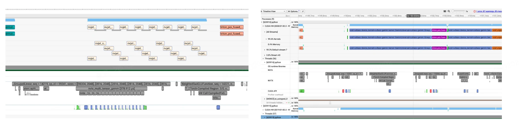
前面我们已经讨论了 MoE 负载均衡算法与 expert dispatch 的 CUDA Graph 兼容实现,本节来看看 Megatron-LM 是如何实现 Full CUDA Graph 的。
捕获粒度:整个 forward_backward_func
一个自然的问题是:Megatron 的 Full CUDA Graph 是否支持 Pipeline Parallelism(PP)?
答案是支持的。Full CUDA Graph 捕获的是整个 forward_backward_func 的执行,而不是单个 layer 或单个 stage。forward_backward_func 内部会处理所有 PP stages 的前向传播、反向传播,以及 microbatch 的调度(如 1F1B 调度)。因此,一个 CUDA Graph 就包含了:
- 所有 PP stages 的计算
- 所有 microbatches 的处理
- PP stages 之间的通信(send/recv)
具体来看,CUDA Graph 的捕获发生在 warmup 步骤完成之后。在捕获时,所有进程通过 torch.distributed.barrier() 同步,然后使用 torch.cuda.graph() 上下文管理器捕获整个 forward_backward_func 的执行:
        if curr_iteration == self.cuda_graph_warmup_steps:
            logger.info(f'Capture CUDA graph for {training_str}!!!')
            torch.distributed.barrier()
            assert FullCudaGraphWrapper.cuda_graph[training_str] is None
            FullCudaGraphWrapper.cuda_graph[training_str] = torch.cuda.CUDAGraph()
            # ... 注册 RNG states
            with torch.cuda.graph(
                FullCudaGraphWrapper.cuda_graph[training_str],
                stream=capture_stream,
                capture_error_mode="thread_local",
            ):
                # 捕获整个 forward_backward_func,包含所有 PP stages
                FullCudaGraphWrapper.result[training_str] = self.forward_backward_func(
                    *args, **kwargs
                )
数据读取:支持多 stage PP
同时我们也能看到,data_read 方法在数据读取上天然支持多 stage PP。它会根据 PP stage 数量,为每个 stage 分别读取 microbatch 数据,并将其复制到静态缓冲区中(这是 CUDA Graph replay 所必需的):
    def data_read(self, data_iterator, model, training, num_microbatches):
        """Read all microbatch inputs from Dataloader and copy to static buffers."""
        if not isinstance(model, list) or len(model) == 1:
            # 单 stage 场景(无 PP 或 PP size = 1)
            assert not isinstance(data_iterator, list) or len(data_iterator) == 1
            # ... 处理单个 data_iterator
        else:
            # 多 stage 场景(PP size > 1)
            assert isinstance(data_iterator, list) and len(data_iterator) == len(model)
            data_list = []
            for i in range(len(model)):
                if data_iterator[i] is not None:
                    # 为每个 PP stage 分别读取 microbatch 数据
                    data_list_i = []
                    for b in range(num_microbatches):
                        data_list_i.append(...)
                    data_list.append(iter(data_list_i))
                else:
                    data_list.append(None)
因此,无论 PP 有多少个 stage,整个系统只会创建 2 个 CUDA Graph:1 个用于 training,1 个用于 validation。这种设计极大地简化了 CUDA Graph 的管理复杂度。
Device-Initiated Grouped GEMM 消除同步
TE 的两种 grouped GEMM 后端
在 MoE 架构中,Router 会将不同的 token 路由到不同的 expert,因此每个 expert 接收到的 token 数量各不相同。这意味着我们不能简单地使用一个统一大小的矩阵乘法(GEMM),而是需要执行一组大小各异的 GEMM——即 grouped GEMM。在 Megatron-LM 中,通常通过调用 Transformer Engine(TE)的 grouped GEMM 来完成这一计算,具体是调用 TE 的 pytorch.GroupedLinear 类。
TE 实现 grouped GEMM 主要通过两种后端:
- cuBLAS 后端:当前 cuBLAS 实际上并没有提供真正的单次 kernel launch grouped GEMM 接口。TE 的做法是循环调用多次 cuBLAS kernel,并将它们分发到不同的 CUDA stream 上并行执行(见下图左侧)。这种 multi-stream 方式虽然能实现并行,但我们观察到在 B 系列 GPU 上 kernel launch 的 overhead 依然很大,不同 stream 之间并没有很好地 overlap 起来。
- CUTLASS 后端:CUTLASS 原生支持单次 kernel launch 的 grouped GEMM(见下图右侧),所有 expert 的计算在一次 kernel 调用中完成,减少了 launch 开销。
我们可以通过环境变量 NVTE_USE_CUTLASS_GROUPED_GEMM 来控制使用 cuBLAS 还是 CUTLASS 后端。但在 TE 2.12 版本中,这个环境变量仅对 H 系列 GPU(Hopper)生效,在 B 系列(Blackwell)上即使设置了也会 fallback 到 cuBLAS。值得注意的是,在 H 系列芯片上 multi-stream 方式的性能反而更优,而在 B 系列芯片上 cuBLAS 同样更快。因此,我们后续讨论的实现方案以 cuBLAS 作为后端。
GPU-CPU 同步的根因:torch.split
尽管 cuBLAS 后端在性能上有优势,但 TE 2.12 在启动 grouped GEMM 时会触发一次关键的 GPU-CPU 同步,其根源在于 torch.split 这个 API。在 TE 2.12 的代码中,有这样一行:
inputmats = torch.split(cast_if_needed(inp_view, activation_dtype), m_splits_list)
torch.split 要求 m_splits_list 参数必须是 CPU 上的 Python list。它会将输入 tensor inp_view 按照 m_splits_list 中指定的大小切分成多个子 tensor,每个子 tensor 对应一个 expert 的输入。
而 m_splits_list 就是 tokens_per_expert——每个 expert 分到的 token 数量。这个信息最初是在 GPU 上通过 routing 计算得到的,因此在 Megatron-LM 中,需要通过 .cpu().tolist() 将 GPU tensor 转换为 CPU 上的 Python list。正是这个 .cpu() 操作触发了隐式的 GPU-CPU 同步——CPU 必须等待 GPU 上所有先前提交的操作完成,才能读取到正确的 tokens_per_expert 值。
从另一个角度看,在 TE 2.12 版本中,m_splits 虽然作为参数传递到了 C++ 层面的 te_general_grouped_gemm,但实际上并未被使用——因为切分信息已经通过 torch.split 编码在了 A[i].shape[0] 中。这意味着 m_splits 这个变量是完全冗余的。
解决方案:GPU 端参数设置 kernel
在 CUDA Graph 的要求下,我们不能有任何 GPU-CPU 同步。因此,我们需要想办法将 torch.split 完全搬到 GPU 上。解决思路是将 m_splits 始终保留在 GPU 上,通过一个轻量级 GPU kernel 完成原本由 torch.split 承担的参数配置工作。
具体实现可以参考这个文件,它完成了 TE 2.12 尚未实现的两项关键功能:
- 在 B 系列(Blackwell/SM100)上支持 CUTLASS 作为 grouped GEMM 后端
- 消除 CPU-GPU 同步,完全在 GPU 端完成类似
torch.split的功能
对于第 2 点,核心思想是在启动 CUTLASS Grouped GEMM 之前,先启动一个轻量级 GPU kernel(setGroupedGemmArguments_fp16bf16),它直接从 GPU 内存中读取 m_splits 并配置每个 expert 的 GEMM 参数。整个过程无需 CPU 参与,因此不会触发 CPU-GPU 同步,使得 MoE 层可以完全被 CUDA Graph 捕获:
__global__ void setGroupedGemmArguments_fp16bf16(int num_experts, const int64_t *gemm_m_per_expert,
                                        int gemm_n, int gemm_k, ElementA *ptr_A, ElementD *ptr_D,
                                        UnderlyingProblemShape *problem_sizes,
                                        ElementA **ptr_A_list, StrideA *stride_A_list, StrideB *stride_B_list,
                                        ElementD **ptr_D_list, StrideD *stride_D_list) {
  uint64_t m_offset = 0;
  if (threadIdx.x == 0 && blockIdx.x == 0) {  // 只用一个线程执行
    for (int expert_id = 0; expert_id < num_experts; expert_id++) {
      int gemm_m = int(gemm_m_per_expert[expert_id]);  // <-- 直接从GPU读取m_splits
      problem_sizes[expert_id] = cute::make_shape(gemm_m, gemm_n, gemm_k);

      ptr_A_list[expert_id] = ptr_A + m_offset * gemm_k;  // 计算每个expert的A指针
      stride_A_list[expert_id] = cute::make_stride(int64_t(gemm_k), _1{}, _0{});
      // ...
      ptr_D_list[expert_id] = ptr_D + m_offset * gemm_n;  // 计算每个expert的D指针
      stride_D_list[expert_id] = cute::make_stride(int64_t(gemm_n), _1{}, _0{});

      m_offset += gemm_m;  // 累加偏移
    }
  }
}
对于第 1 点(在 B 系列上实现 CUTLASS grouped GEMM),相关函数 generic_moe_gemm_kernelLauncher_fp16bf16 的实现主要分为 4 个阶段:
- 阶段 1:定义 CUTLASS 类型。使用 CUTLASS 的 Builder 模式定义高性能 Grouped GEMM kernel 的所有类型参数,包括矩阵元素类型、布局、Tile 大小和调度策略等。
// 定义 GEMM 问题形状
using ProblemShape = cutlass::gemm::GroupProblemShape<Shape<int, int, int>>;  // <M,N,K>

// 配置矩阵类型和布局
using ElementA = ElementInput;  // FP16 或 BF16
using LayoutA = cutlass::layout::RowMajor;
using ElementAccumulator = float;  // 累加器用 FP32

// 核心配置:针对 SM100 (Blackwell) 架构
using ArchTag = cutlass::arch::Sm100;
using MmaTileShape = Shape<_256, _256, Int<128 / sizeof(ElementA)>>;  // Tile 大小
using KernelSchedule = cutlass::gemm::KernelPtrArrayTmaWarpSpecialized2SmSm100;  // TMA调度

// 构建 GEMM kernel
using GemmGrouped = cutlass::gemm::device::GemmUniversalAdapter<GemmKernel2SM>;
- 阶段 2:Workspace 内存布局。在预分配的 GPU workspace 中划分内存区域,用于存储各 expert 的 GEMM 参数。这些参数将在阶段 3 中由 GPU kernel 填充。
// 在 workspace 中分配各种指针数组和 stride 数组
auto ptr_A_list = ...;     // 每个 expert 的 A 矩阵指针
auto ptr_D_list = ...;     // 每个 expert 的 D(输出)矩阵指针
auto stride_A_list = ...;  // 每个 expert 的 A stride
auto stride_B_list = ...;  // 每个 expert 的 B stride
auto stride_D_list = ...;  // 每个 expert 的 D stride
auto problem_sizes = ...;  // 每个 expert 的 GEMM shape (M, N, K)
- 阶段 3:启动参数设置 Kernel。这是消除 CPU-GPU 同步的关键步骤。启动一个轻量级 GPU kernel,在 GPU 上直接读取
gemm_m_per_expert(即m_splits),并填充每个 expert 的 GEMM 配置: - problem_sizes[i] = (M_i, N, K) —— 每个 expert 的 GEMM 形状
- ptr_A_list[i] —— 每个 expert 的输入指针
- ptr_D_list[i] —— 每个 expert 的输出指针
- 各种 stride
setGroupedGemmArguments_fp16bf16<<<1, 32, 0, stream>>>(
    num_experts, gemm_m_per_expert,  // <-- m_splits (GPU tensor)
    gemm_n, gemm_k, ptr_A, ptr_D, problem_sizes,
    ptr_A_list, stride_A_list, stride_B_list,
    ptr_D_list, stride_D_list);
- 阶段 4:启动 CUTLASS Grouped GEMM。使用阶段 3 在 GPU 上设置好的参数,启动 CUTLASS Grouped GEMM kernel。由于所有参数都已在 GPU 端准备就绪,整个过程不需要任何 CPU-GPU 同步。
// 构建 CUTLASS 参数
args = typename GemmGrouped::Arguments{
    cutlass::gemm::GemmUniversalMode::kGrouped,
    {num_experts, problem_sizes, nullptr},  // 问题形状(在 GPU 上)
    {ptr_A_list, stride_A_list, ptr_B_list, stride_B_list},  // 输入
    {fusion_args, nullptr, stride_D_list, ptr_D_list, stride_D_list},  // 输出
    hw_info, scheduler
};

// 初始化并运行
gemm.initialize(args, workspace + offset);
gemm.run(stream);  // 执行 Grouped GEMM